Contents

% /home/dimarzio/Documents/working/12303/matlab/ftclass2018.m
% Sun Nov  4 13:24:51 2018

Class exercise

% You will need to download
% fftaxis.m
% fftaxisshift.m
% cxplot.m
% xzoom.m

% Run the code snippet below and follow the instructions below it.

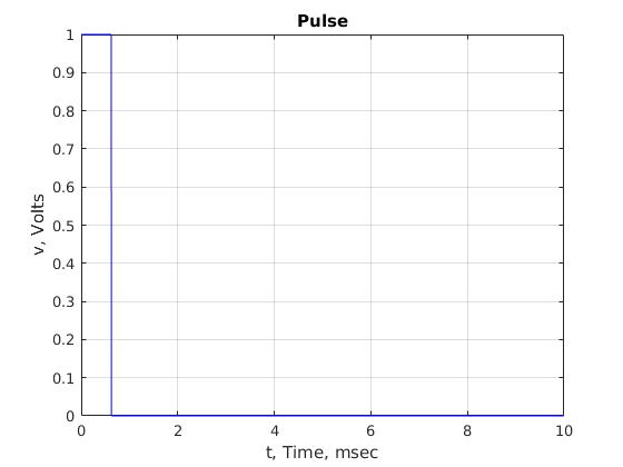
A pulse

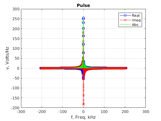
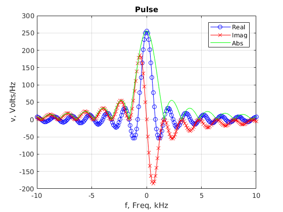
t=[0:4096-1]*10e-3/4096;  % Time axis
v1=zeros(size(t));
v1(1:256)=1;
figure;plot(t*1e3,v1,'b-');grid on;
title('Pulse');
xlabel('t, Time, msec');ylabel('v, Volts');

f=fftaxisshift(fftaxis(t));
V1=fftshift(fft(v1));

figure;cxplot(f/1e3,V1);grid on;
title('Pulse');
xlabel('f, Freq, kHz');ylabel('v, Volts/Hz');

% zoom to center
figure;cxplot(f/1e3,V1);grid on;
xzoom(-10,10);
title('Pulse');
xlabel('f, Freq, kHz');ylabel('v, Volts/Hz');

Time shift

dt=t(512);

% Use the equation for a time shift in the frequency domain (V1) to
% shift v1 by the time dt.  Call the new spectrum V2 and the new
% time history v2. Plot V2 and v2 with appropriate axes and title.
% Plot only the useful part using xzoom as I did above.

Square in the frequency domain.

% Square V2 in the frequency domain. Call it V3. Plot it.
% Transform to the time domain, v3, and plot it. Again, use
% appropriate axis lables.

Document your results.

% publish('fftclass.m','pdf');
% print the file html/fftclass.pdf

Published with MATLAB® R2017a